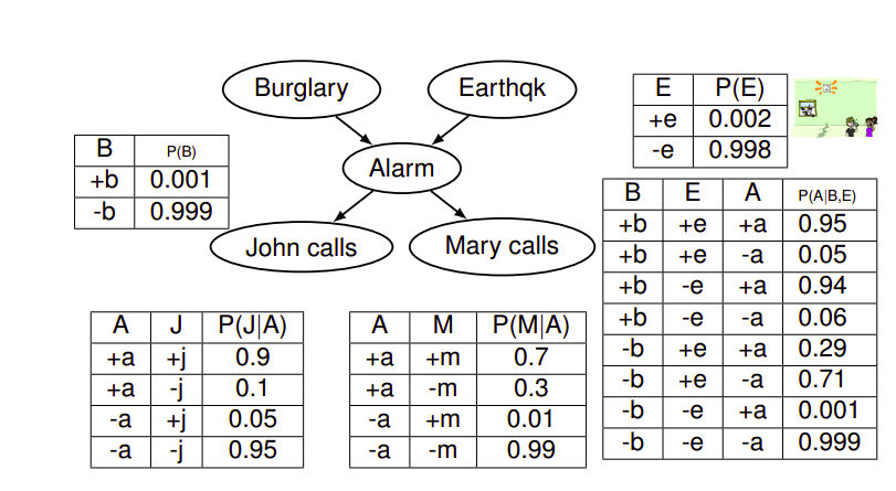
Bayesian Networks

A method used to represent Joint Distributions implicitly using conditional independence and local interactions.

Representation

It is represented as a directed acyclic graph. Each variable is a Node, and a directed edge from node A to node B means that the random variable B is a function of random variable A. In other words, a random variable is a function of the random variables in its parent nodes.

Every node A stores a table that represents the conditional probability of random variable A given every combination of values its parents could take.

From Conditional to Joint

In order to extract the joint distribution from the local conditionals, we can use the following formula:

Size of a Bayesian Network

In order to store a table that represents an ordinary joint distribution of N variables where each variable can take d values, one would need $O(d^N)$ entries which is too large.

One important advantage of Bayesian Networks is that they reduce this size needed to store a join distribution by storing different small parts from which we can reconstruct the joint distribution. Every node contains a table that determines its value for every combination of values of its parents. If we assume that every node has no more than k parents, this would mean that every node has a table of size $O(d^{k+1})$ ($k + 1$ comes from the fact that we encode the parents and the node itself), so for N nodes, we would get a total of $O(Nd^k)$, which is a reduction that depends on k, the maximum number of possible parents.

Does a Bayesian Network Graph imply Causality ?

No, not all the time. It is easier to think of the graph as if it means that a certain variable (parent) is causing another variable (child), but that is not always the case. Rather, it only means that there is a direct conditional dependency between variables.

How to check for Independence in a Bayesian Networks

If two variables do not have a direct connection, this does not mean that they are independent, they might indirectly influence each other through other nodes.

For example in this graph below, A and B are not necessarily independent because they can influence each other through B.

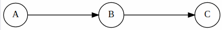
Nevertheless, we can prove conditional independence of some cases. For example, in the network above, we can say that C is conditionally independent from A given B. The intuition is that since a value of B was given, it already holds the influence from A, or another way to think of it that the influence between A and C was blocked by B.

There are 3 types of simple 3-node graphs which are simple to analyze and will be used to detect properties in Bayesian Networks. These graphs are causal chains, common cause, and common effect.

Causal Chains

From this structure we can only say that C is conditionally independent of A given B. (can be proven mathematically)

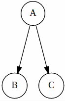
Common Cause

Here, we can say that B and C are independent given A. (can be proven mathematically)

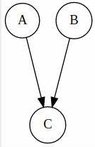
Common Effect

Here, A and B are in fact fully independent, but they are not independent given C.

Detect if 2 nodes are conditionally independent from the graph structure

We can do this by tracing the undirected path between any two nodes on the graph. For every 3 consecutive nodes on the path, we check if they satisfy conditional independence. In order to do the check, we simply identify to which type this triplet belongs (causal chain, common cause, common effect). If we find any triplet on the path to voilate independence then we assume that conditional independence between source and target node is not guaranteed. The triplets which imply conditional independence are called Inactive Triplets, whereas triplets that violate conditional independence are called Active Triplets. The following figure summarizes the triplet cases.

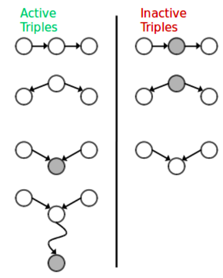
This approach is called D-Separation.

Markov Blanket

For a given node X, we can say that it is conditionally independent of all other nodes given its Markov Blanket. A Markove Blanket for a node consists of its parents, children, and children’s parents. Like in the image below.

Probabilistic Inference

The act of calculating the probability that some random variables take certain values from a join distribution.

Inference by Enumeration

This is basically the brute force way of calculating a certain probability, where we first take the sum of the probabilities of all the hidden random variables to eliminate them, and then calculate the desired probability of the target and evidence.

Note: Hidden variables are the rest of the random variables which are neither in the target set, nor in the evidence set. Evidence contains the random variables which make the condition of the probability calculated.

Enumeration gives an exact answer but is exponential in complexity.

Steps of performing Inference by Enumeration

1. From each probability table, select the entries whose rows are consistent with the evidence. That is, if we have two variables A and B in the evidence, and both take values a and b respectively, then select all rows for which variables A and B have values a and b respectively.
2. For all the hidden variables, sum out their values. This means compute the sum of probabilities for all combinations of hidden variables values. This operation is called marginalization. \(P(Q, e_1 \dots e_n) = \sum_{h_1 \dots h_r} P(Q, h_1 \dots h_r, e_1 \dots e_k)\)
3. Normalize the the the values left so that their sum is 1 and they form a valid distribution.

Variable Elimination

In enumeration, what we did was build the whole join distribution and then marginalize in order to reduce it to the desired state of target and evidence variables. The idea suggested by Variable Elimination to speed up the calculations is to interleave between joining and marginalizing. It basically remains exponential but it helps speed up the calculations compared to enumerations.

In order to understand how Variable Elimination works, we need to understand the concept of Factors first.

Factors

Factorization as a mathematical concept means to decompose an object into a product of other objects called factors.

Note: Capital letters in a distribution determine its dimensions, because small letters denote assigned values.

For Bayesian Networks, let’s see what kind of factors there can be:

• Joint Distribution $P(X,Y)$
  • Contains entries $P(x,y)$ for all $x,y$
  • Sums to 1
• Selected Joint $P(x, Y)$
  • A slice of the joint Distribution
  • Sums to $P(x)$, because it represent probability of $x$ for every value of $y$, which means that $P(x)$ is sort of partitioned over $y$ values.
• Single Conditional $P(Y|x)$
  • Contains entries $P(y, x)$ for all $y$ and fixed $x$
  • Sums to 1, because it is basically a conditional probability distribution for all values of y conditioned on a single value $x$.
• Family of Conditionals $P(Y|X)$
  • Contains multiple conditionals.
  • Contains Entries $P(y|x)$ for all $x,y$
  • sums to $|X|$, which is the number of values that can be taken by the random variable $X$. This is because for every value $X$, we have a conditional distribution for $Y$ over that particular $x$, which means we essentially have $|X|$ distributions where each one sums to 1.
  • Specified Family $P(y|X)$
    • Contains entries $P(y|x)$ for fixed $y$, but for all $x$.
    • Sums to an unknown value.

So now back to Variable Elimination, we will use 2 main operations, join and eleminate. Join operation basically joins two tables in a similar way to the database join operations. In simpler terms, if table A has two variables X and Y, and table B has two variables Y and Z, then a join operation would result in a 3 dimensional table of X, Y, and Z. where probability of an entry in table A is multiplied by the a probability of table B where the common variable Y values match. Eliminate operations is simply summing for all the values of a certain variable to remove it from the table.

1. Select all rows that match the evidence and delete rows that do not match it, that is only if a table contains an evidence variable. If a table does not contain an evidence variable don’t touch it. Here are the steps to follow in order to solve a query using Variable Elimination:
2. Since we cannot eliminate a hidden variable unless it exists in only one facts, we join factors which have a common hidden variable.
3. Then for every factor which contains a hidden variable and that hidden variable only exists in that factor, eliminate the hidden variable.
4. Repeat steps 2 and 3 until the factor left consists of target and evidence.
5. Finally we normalize the table we get, because the existence of evidence variables might cause a selected joint to appear.

Note: When joining two tables where each table contains some variables on the left side of the condition and variables on right side, the trick is to place all variables on the left side of the two tables to the left side of the output table, and then place the rest on the right. This would save time in a case where a variable exists on the left side of a table and the right side of another table. To understand what I mean by left and right: $P(X|Y)$, here $X$ is the left of the condition and $Y$ is the right of the condition.

Conclusion of Variable Elimination: The worst case complexity of Variable Elimination is not better than Enumeration in theory but in practice it is faster. This difference in speed is due to the fact that eliminating some variables in a certain order decreases the maximum factor generated, which affects the computations significantly if we were able to find a good ordering.

Approximate Inference

Since it takes too long to calculate exact inferences using the method discussed earlier, we may sacrifice some of the exactness in order to speed up the calculation. One method to do this is Sampling.

Sampling

The idea behind sampling is to draw $N$ samples from a distribution and then use these samples to compute an approximate posterior probability and show that this can converge to the true probability. How can we computer a posterior probability from samples ? Simply, we divide the number of samples matching the target over the samples matching the evidence, a very basic way of calculating probability.

How to sample from a known distribution

Since it is a known distribution, then for each value the random variable takes we know its probability. Hence, we do the following steps:

1. Get a sample $u$ from the uniform distribution over the interval [0, 1) (assume that we have the mechanism to do so).
2. For every value of the random variable assign an interval in the range [0, 1) which is of length equal to the probability at that value. We can do this because the sum of all probabilities is equal to 1.
3. Choose the value of the random variable that has the sample $u$ within it.
4. Repeat this process $n$ times to get $n$ samples.

Four main sampling methods will be discussed

• Prior Sampling
• Rejection Sampling
• Likelihood Weighting
• Gibbs Sampling (Most used)

Prior sampling

To apply prior sampling on a Bayesian Network:

1. Sort the nodes in the graph using topological sorting.
2. Iterate over the variables in the sorted order and randomly sample from each. Sampling from a node would affect sampling of its children, because if a random variable A gets a value a, then when sampling from its child B, we sample from the distribution that is conditioned on A taking the value a. Topological sorting guarantees that a node will not be sampled until all its parents are sampled, which determines the value combinations the child needs to sample from.
3. When the last node is reached, we would have gained a single sample of our Bayesian Network. So we need to repeat the steps $n$ times to get $n$ samples.
4. Once we get $n$ samples, we eliminate the samples which do not match the evidence, then the desired probability would be the number of samples which match the target divided by the number of samples left.

As $n$ goes to infinity, then the probabilities computer using Prior Sampling would converge to the exact original probabilities. This is why we call this sampling method consistent.

Rejection Sampling

The idea in Rejection Sampling is simple, given a desired query with targets and evidence, for every sample we get, we reject it if it does not match our desired evidence. That is, if we want to collect $n$ samples, we keep drawing samples such that all the $n$ chosen samples have our evidence satisfied, so we might perform more than $n$ sampling operations to get $n$ samples which match our evidence. The number of sampling operations can be very high if our evidence is unlikely because we would reject many of the samples we get.

Likelihood Weighting

Rejection Sampling has a very serious limitation, which is the fact that many samples can be rejected if the evidence was unlikely. Likelihood Weighting solves this issue with the following steps:

1. Fix the evidence variables and sample from the others instead of rejecting.
2. Fixing evidence alone would disrupt the distribution and make it inconsistent. Therefore, we modify the sampling algorithm maintain and return a constant weight which is initially set to 1.
3. As we move through the network in topological order, if we encounter an evidence variable, we multiply its probability give its parents with the weight constant we have and update the value of the weight to the new value (old value times probability of evidence given its parents).
4. The sampling algorithm returns the sample with accumulated weight, so in this way every sample will be associated with a certain weight.

Likelihood Weighting is consistent because the product of Sampling distribution that is a result of fixing evidence and the weight of every sample (which is an accumulated product of evidence variables given their parents) gives us the original join distribution (Mathematical equations to be added here later).

Note: After generating the samples, instead of counting the number of samples satisfying the target, we sum the weights instead. This is essential to produce a consistent answer.

Issues of Likelihood Weighting: Fixing the evidence affects the downstream variables (variables which are reachable from an evidence in the directed graph and come after it in the topological sorting), but it does not affect the upstream variables (variables which can reach the evidence in the directed graph and come before it in the topological sorting). this is bad because when fixing the evidence, all its downstream will be affected by its value but it would still follow the distribution. On the other hand, fixing the value of an evidence regardless of its parents values creates an inconsistency which we approximately solve by using the weight approach. Therefore, the larger the number of upstream variables, the less accurate the approximation is. Following this logic, we prefer evidences that exist at the top of the hierarchy rather than the bottom.

Gibbs Sampling

Gibbs Sampling addresses the issue with Likelihood Weighting, which is that the upstream variables of a fixed evidence are sampled independently from the fixed evidence. Gibbs Sampling attempts to sample all variables taking evidence into consideration.

Approach to Generate a Single Sample:

1. Start with a random assignment to each variable except for the evidence variables which are already fixed with their pre-determined values.
2. Sample each non-evidence variable one variable at a time (Round Robin Style), conditioned on all the other variables while keeping the evidence fixed.
3. Repeat this for a long time.

This approach has the property that repeating it infinitely many times results in a sample that comes from the correct distribution. This way we also guarantee that both upstream and downstream variables are conditioned on evidence.

One might ask: How efficient is it to sample one variable conditioned on all the rest ? Well, the probability of a variable conditioned on all the rest is equal to the joint probability divided on the probability of all the rest. In this equation many terms would cancel out between the numerator and denominator. More specifically, all Conditional Probability Tables which do not contain the re-sampled variables will be canceled out. In other words, to re-sample a variable we simply join the tables that contain it and use them for the calculations, which can be faster if the local interactions in the Bayesian Network were limited.

Note: Sampling a variable given its Markov Blanket is enough.

As with the previous methods, once we have the samples, probabilities are computer by counting samples that match the target and divide by the number of samples (because they all match the evidence by definition).

Note: Gibbs Sampling is special case of a more general method called Markov Chain Monte Carlo (MCMC) methods. Metropolis-Hastings is another famous MCMC method.

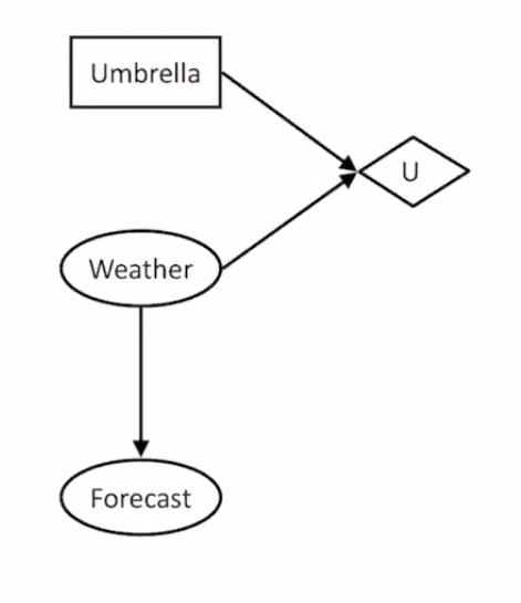
Decision Networks

They are an extension of Bayesian Networks where we assign utilities to outcomes to help make decisions. Two new types of nodes are added to the Bayesian Network:

• Actions (Rectangles): cannot have parents because agents decide on their actions.
• Utility Node (Diamond): depends on action and chance nodes.

How to select an action in this network:

1. Instantiate all evidence variables.
2. Calculate Posterior of all parents of the utility node.
3. For every possible action, calculate the expected utility.
4. Choose Action with maximum utility. This is called the Maximum Expected Utility (MEU).

Value of Information

Finding the value of discovering new information or in the case of Bayesian Network adding new evidence values can help in deciding to which direction we must put effort in order to collect data. Therefore we attempt to calculate the Value of Information to guide our choices and decisions better.

How to calculate the Value of Information ?

1. Calculate the Maximum Expected Utility (MEU) before acquiring the new evidence.
2. Calculate expected MEU after acquiring the new evidence
3. Value of Information is equal to new expected MEU minus old MEU.
4. If Value of Information is positive, then it would by worthwhile adding this evidence.

How to calculate the Expected MEU after acquiring new evidence ?

1. Assume evidence is added
2. For every value of the evidence, calculated expected utility conditioned on that value.
3. For every value of the evidence, multiply probability of evidence with expected utility conditioned on that evidence and sum all these values. The result is the expected MEU.

Properties of Value of Information (VPI):

• Non-negative: we can never get a negative VPI.
• Non-Additive

• Order Independent: If you have two evidences to check their values, it doesn’t matter in which order they are calculated.

Note: $VPI$ stands for Value of Perfect Information.

We can have some shortcuts in calculating VPO through some independence properties:

• If $Parents(U)$ ($U$ is utility node) is independent from a node Z given some evidence, then $VPI(Z | evidence) = 0$